
Utility
Utility nodes remap the values depending upon the node’s algorithm.
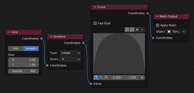
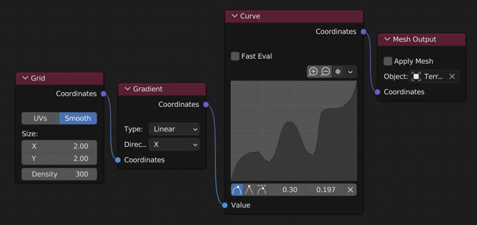
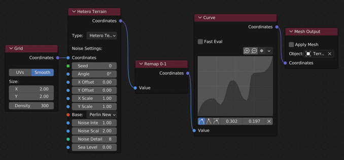
Curve
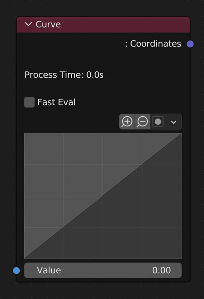
Remap Value to custom curve.
- Fast Eval
- Use a custom multi-threaded formula for evaluating the curve.
- Curve
- The visible result of the function used to remap input values.
- Reload Curve
- Blender doesn’t allow for creating or saving of UI curves. In order to get a node as we have in NodeScapes we create an RGB Curve shader node in a hidden node group. If this node group or the source node is deleted, the curve in the NodeScapes node will disappear and reveal this button. Clicking it will recreate everything it needs to in order to have the curve again. It will also recreate the curve if the curve node had been executed previously.
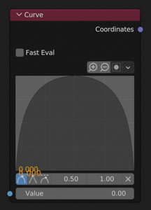
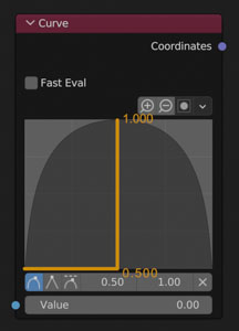
Understanding the Curve Node
The curve node is just a graph. It takes the values (heights) and passes them through the curve. The curve is just a visual representation of a mathematical formula or function or func (y=x, y=2x, y=2x^2, etc.). So if we look at the example curve here we see that if we plug in an input value of 0.0 (y=func(0.0)) we will get an output value of 0.0 because where the x-axis equals 0.0 the y-axis also equals 0.0 on the curve (ex. 1 below). If we plug in 0.5 as the input value (y=func(0.5)) we get an output value of 1.0 because where the x-axis is 0.5 the curve is at 1.0 on the y-axis (ex. 2 below).
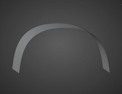
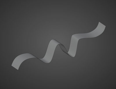
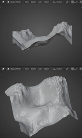
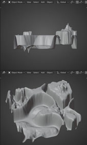
Example
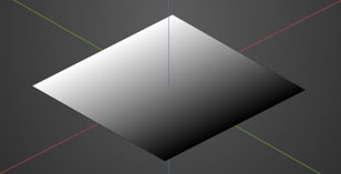
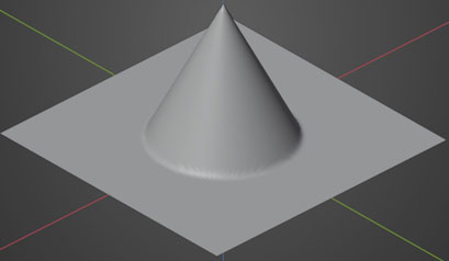
Using a gradient node we can visualize the curve in the geometry.
Remap Value to custom curve.
- Fast Eval
- Use a custom multi-threaded formula for evaluating the curve.
- Curve
- The visible result of the function used to remap input values.
- Reload Curve
- Blender doesn’t allow for creating or saving of UI curves. In order to get a node as we have in NodeScapes we create an RGB Curve shader node in a hidden node group. If this node group or the source node is deleted, the curve in the NodeScapes node will disappear and reveal this button. Clicking it will recreate everything it needs to in order to have the curve again. It will also recreate the curve if the curve node had been executed previously.
Understanding the Curve Node
The curve node is just a graph. It takes the values (heights) and passes them through the curve. The curve is just a visual representation of a mathematical formula or function or func (y=x, y=2x, y=2x^2, etc.). So if we look at the example curve here we see that if we plug in an input value of 0.0 (y=func(0.0)) we will get an output value of 0.0 because where the x-axis equals 0.0 the y-axis also equals 0.0 on the curve (ex. 1 below). If we plug in 0.5 as the input value (y=func(0.5)) we get an output value of 1.0 because where the x-axis is 0.5 the curve is at 1.0 on the y-axis (ex. 2 below).
Example
Using a gradient node we can visualize the curve in the geometry.
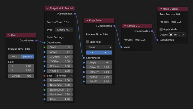
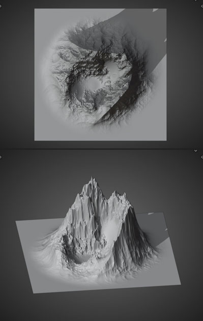
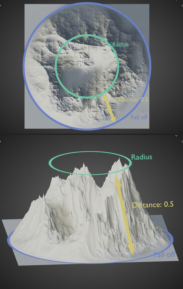
Edge Fade
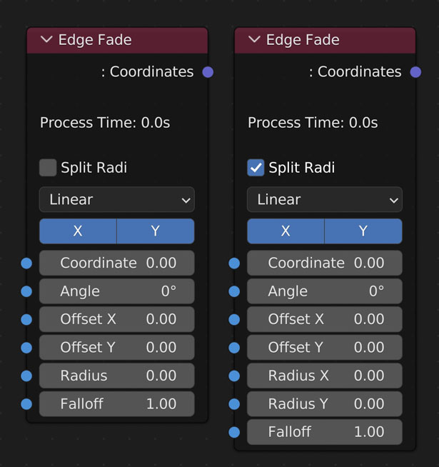
Fade Value to 0 as it gets closer to the edge of the falloff.
- Split Radi
- Split the radius up into X and Y in order to create an ellipse fade off cone
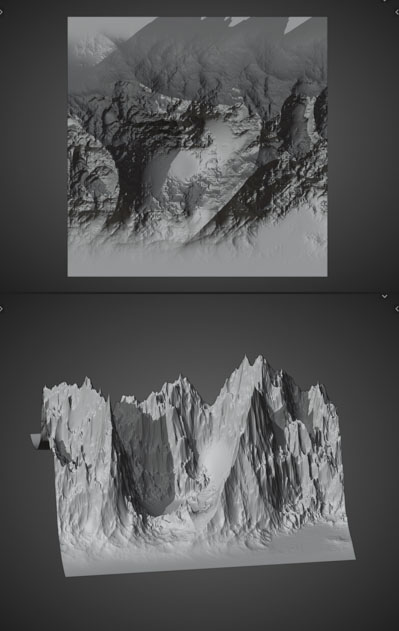
- Fade Type
- Linear: Fades out linearly ( each value is equally less than the one before)
- Ease: Eases in and out
- Ease More: Greater ease in and out
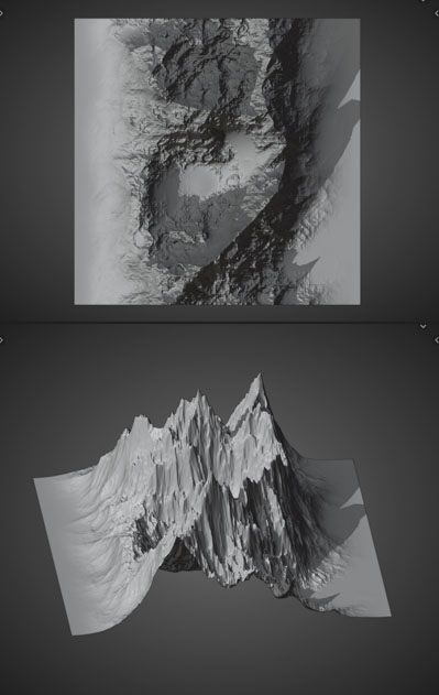
- Fade Direction
- X or Y
- Coordinates
- The coordinates you want to fade out
- Angle
- Rotate the fade direction
- Offset (X, Y)
- Moves center of Fade relative to the center of the object
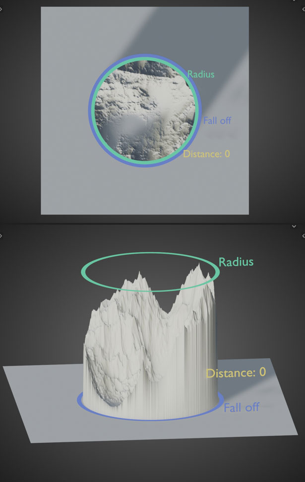
- Radius
- Distance in Blender units to start fading - Falloff
- Distance away from the Radius in Blender units to reach 0
Example
Base
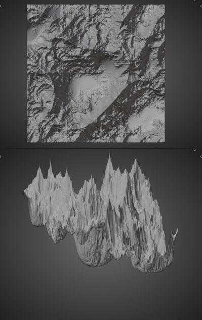
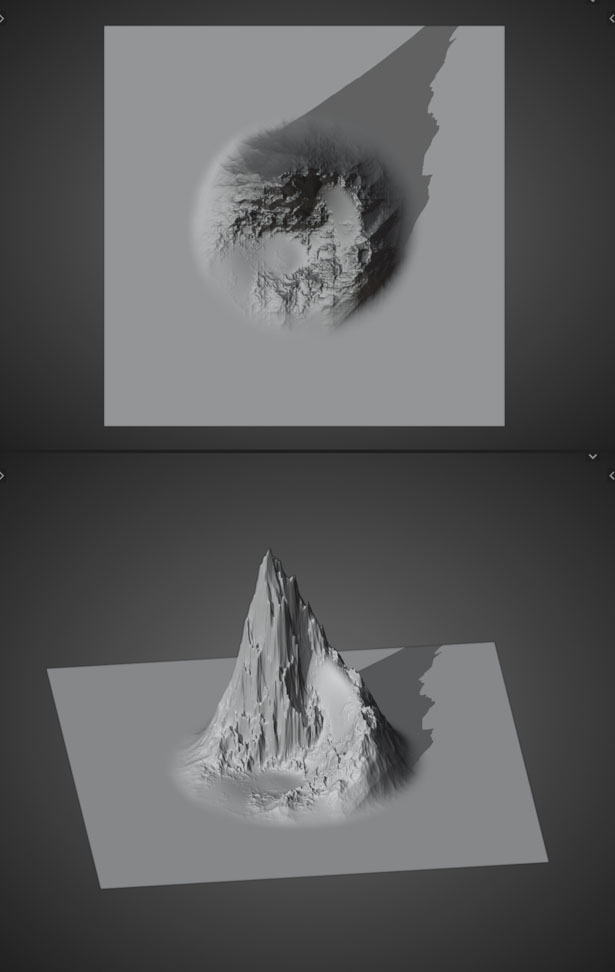
Fade Type
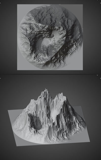
Fade Direction


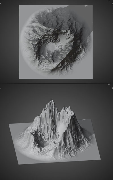
Radius/Falloff
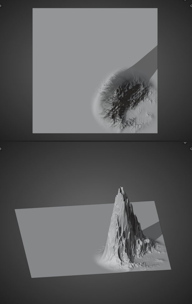
Offset
Split Radi
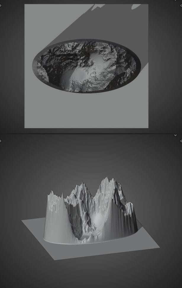
Angle
Fade Value to 0 as it gets closer to the edge of the falloff.
- Split Radi
- Split the radius up into X and Y in order to create an ellipse fade off cone
- Fade Type
- Linear: Fades out linearly ( each value is equally less than the one before)
- Ease: Eases in and out
- Ease More: Greater ease in and out
- Fade Direction
- X or Y
- Coordinates
- The coordinates you want to fade out
- Angle
- Rotate the fade direction
- Offset (X, Y)
- Moves center of Fade relative to the center of the object
- Radius
- Distance in Blender units to start fading - Falloff
- Distance away from the Radius in Blender units to reach 0
Example
Base
Fade Type
Fade Direction
Radius/Falloff
Offset
Split Radi
Angle
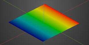
Gradient
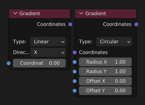
Returns a gradient of selected type from 0-1.
- Type
- Linear
- Create a gradient from 0 to 1 of the given axis (X or Y)
- Direction
- X - Gradate along the X axis
- Y - Gradate along the Y axis
- Circular
- Create a gradient from 0 to 1 in a circular shape with 1 being in the middle and 0 at the edge
- Radius
- X - Sets the circular radius in the X axis
- Y - Sets the circular radius in the Y axis
- Offset
- X - Move the center of the gradient in the X axis
- Y - Move the center of the gradient in the Y axis
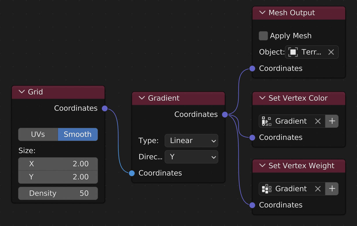
- Coordinates
- Connect the output of the nodes you’d like to use for creating a mask here
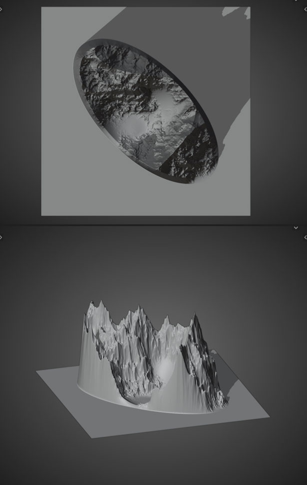
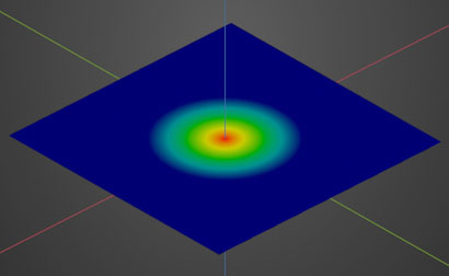
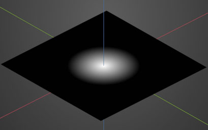
Example:
Linear
X Axis
Y Axis
Circular
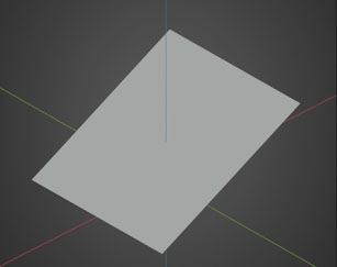
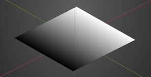
Geometry
Weights
Vertex Colours
Returns a gradient of selected type from 0-1.
- Type
- Linear
- Create a gradient from 0 to 1 of the given axis (X or Y)
- Direction
- X - Gradate along the X axis
- Y - Gradate along the Y axis
- Circular
- Create a gradient from 0 to 1 in a circular shape with 1 being in the middle and 0 at the edge
- Radius
- X - Sets the circular radius in the X axis
- Y - Sets the circular radius in the Y axis
- Offset
- X - Move the center of the gradient in the X axis
- Y - Move the center of the gradient in the Y axis
- Coordinates
- Connect the output of the nodes you’d like to use for creating a mask here
Example:
Linear
X Axis
Y Axis
Circular
Geometry
Weights
Vertex Colours
Interpolate
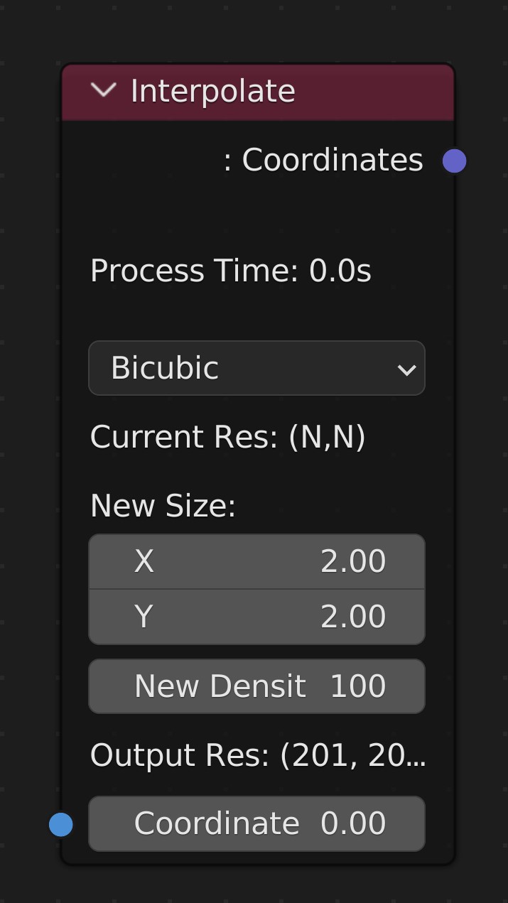
Change the size and density of the current changes
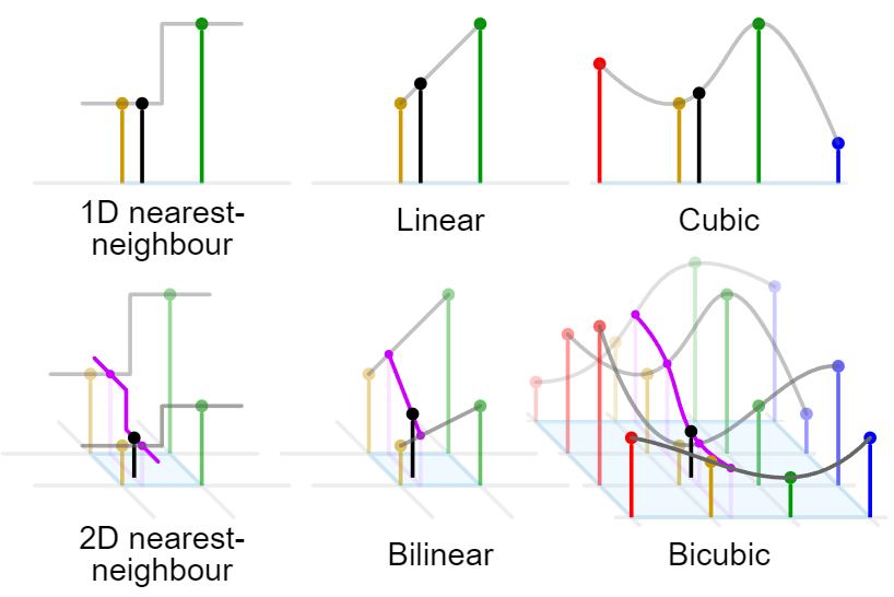
- Interpolation Type
- Nearest Neighbor
- Align vertices to the closest vertex More Info.
- Bilinear
- Smooths from one vertex to the next in a straight line. More Info.
- Bicubic
- Smooths from one vertex to the next in a smooth curve shape. More Info.
- New Size
- The number of Blender Units in the X and Y axes
- New Density
- The number of faces per Blender Unit
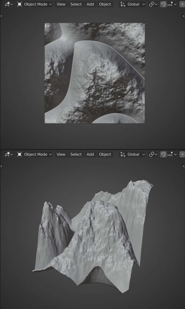
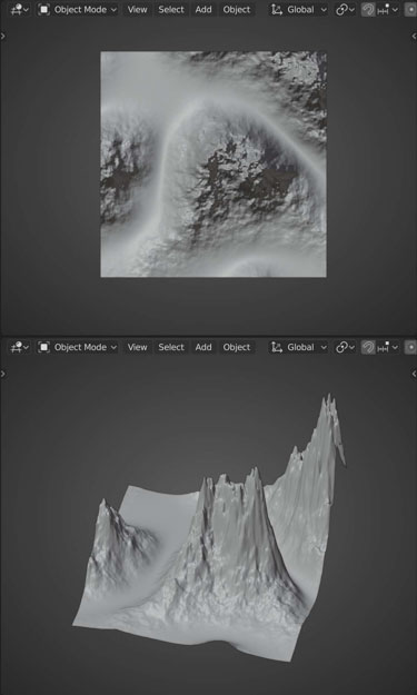
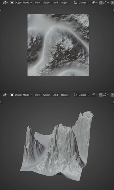
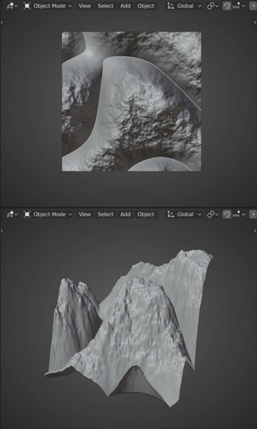
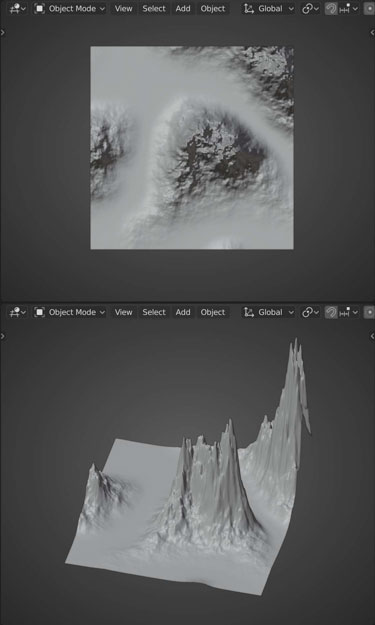
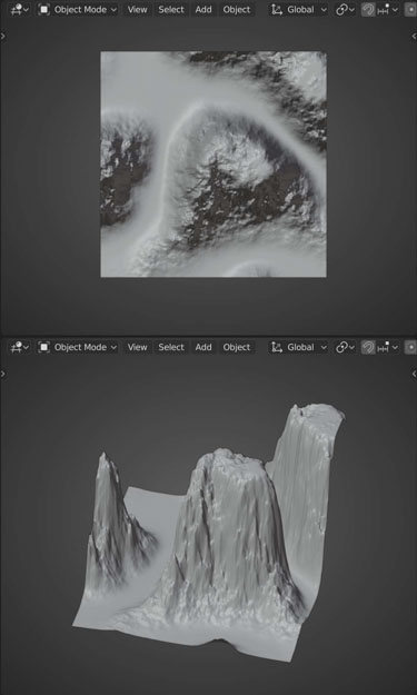
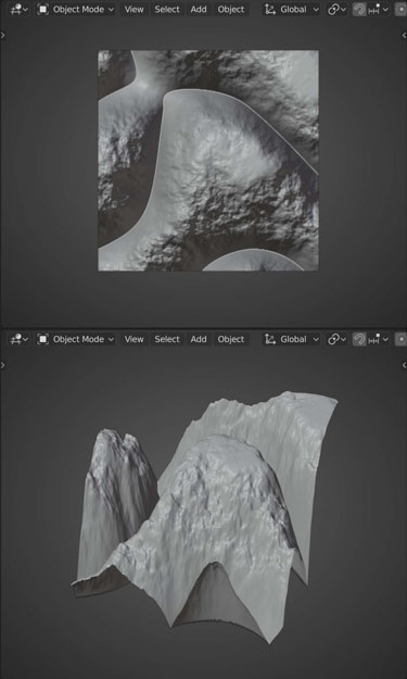
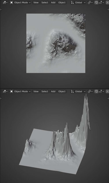
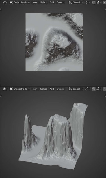
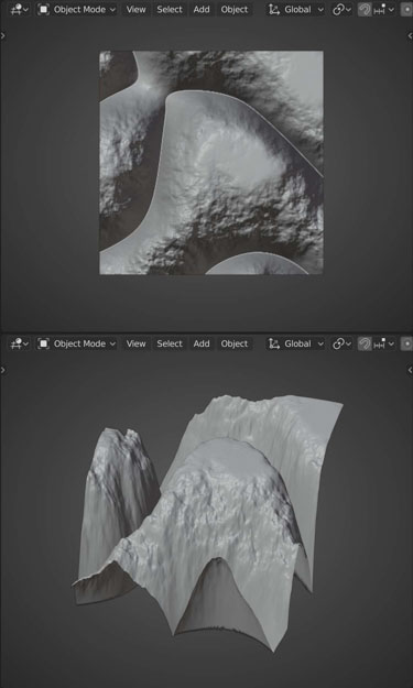
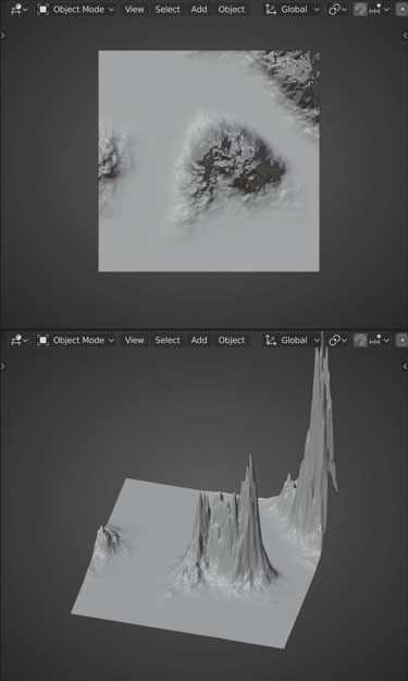
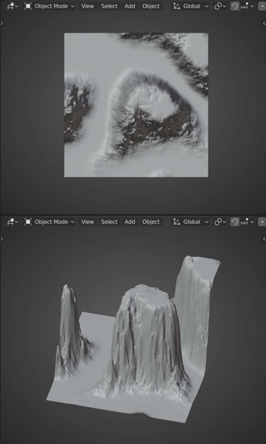
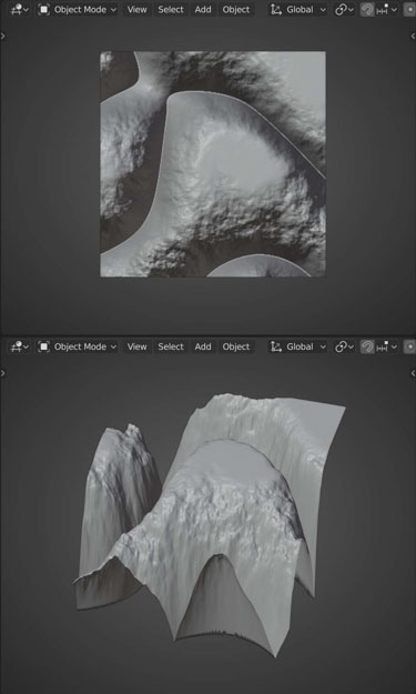
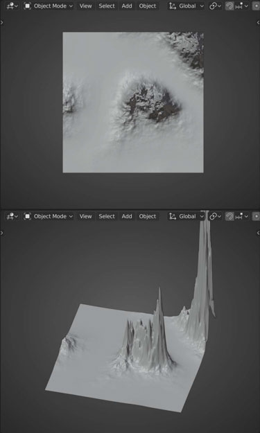
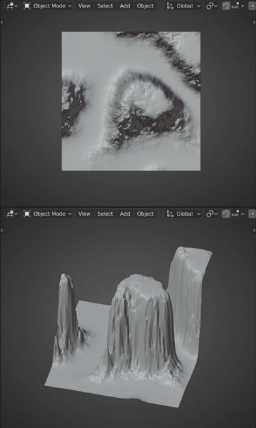
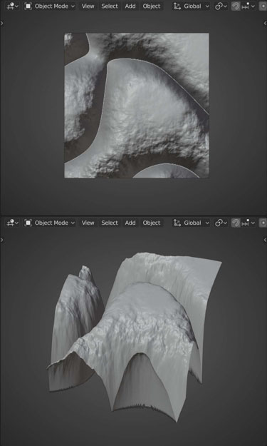
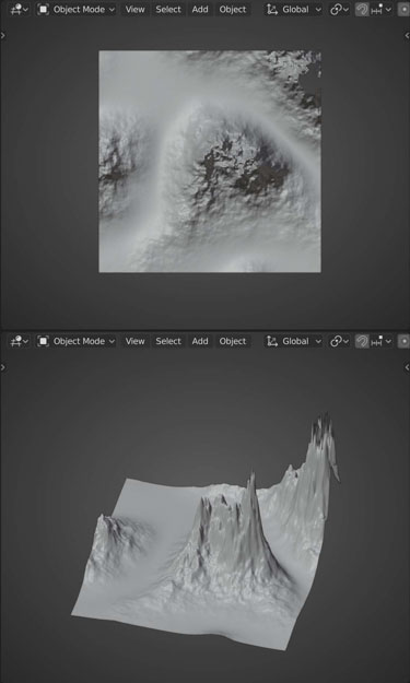
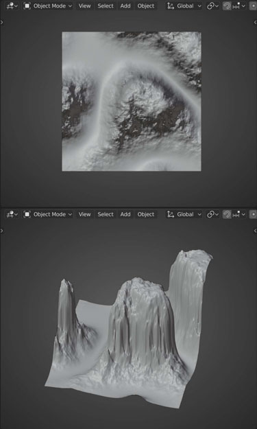
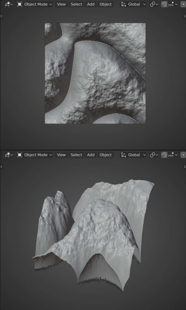
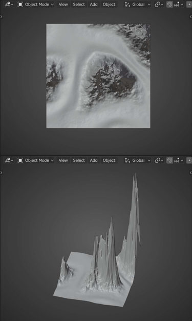
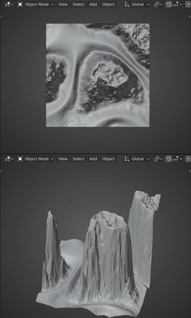
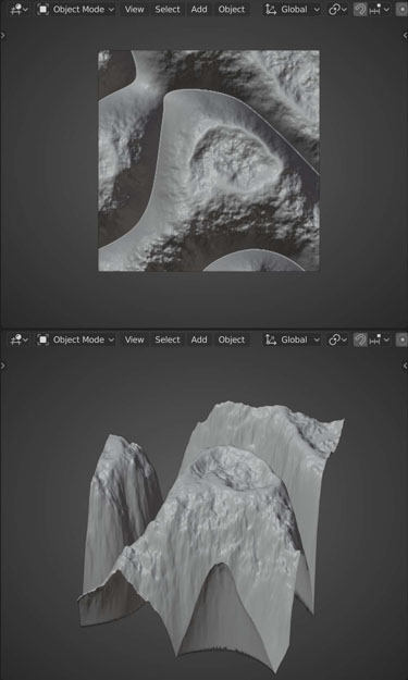
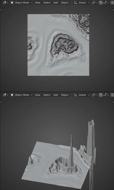
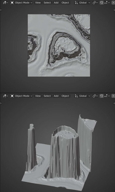
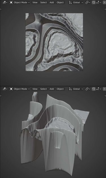
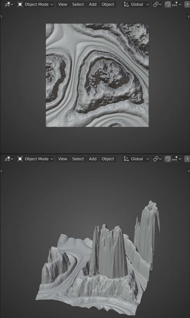
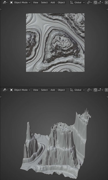
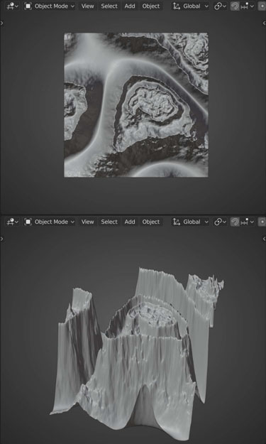
Interpolation Types:
Use:
Using the Hydraulic Erosion node with a lower resolution mesh can give more realistic results, such as more large erosion grooves. Using the Interpolate node afterwards can then provide greater detail for other nodes
Change the size and density of the current changes
- Interpolation Type
- Nearest Neighbor
- Align vertices to the closest vertex More Info.
- Bilinear
- Smooths from one vertex to the next in a straight line. More Info.
- Bicubic
- Smooths from one vertex to the next in a smooth curve shape. More Info.
- New Size
- The number of Blender Units in the X and Y axes
- New Density
- The number of faces per Blender Unit
Interpolation Types:
Use:
Using the Hydraulic Erosion node with a lower resolution mesh can give more realistic results, such as more large erosion grooves. Using the Interpolate node afterwards can then provide greater detail for other nodes
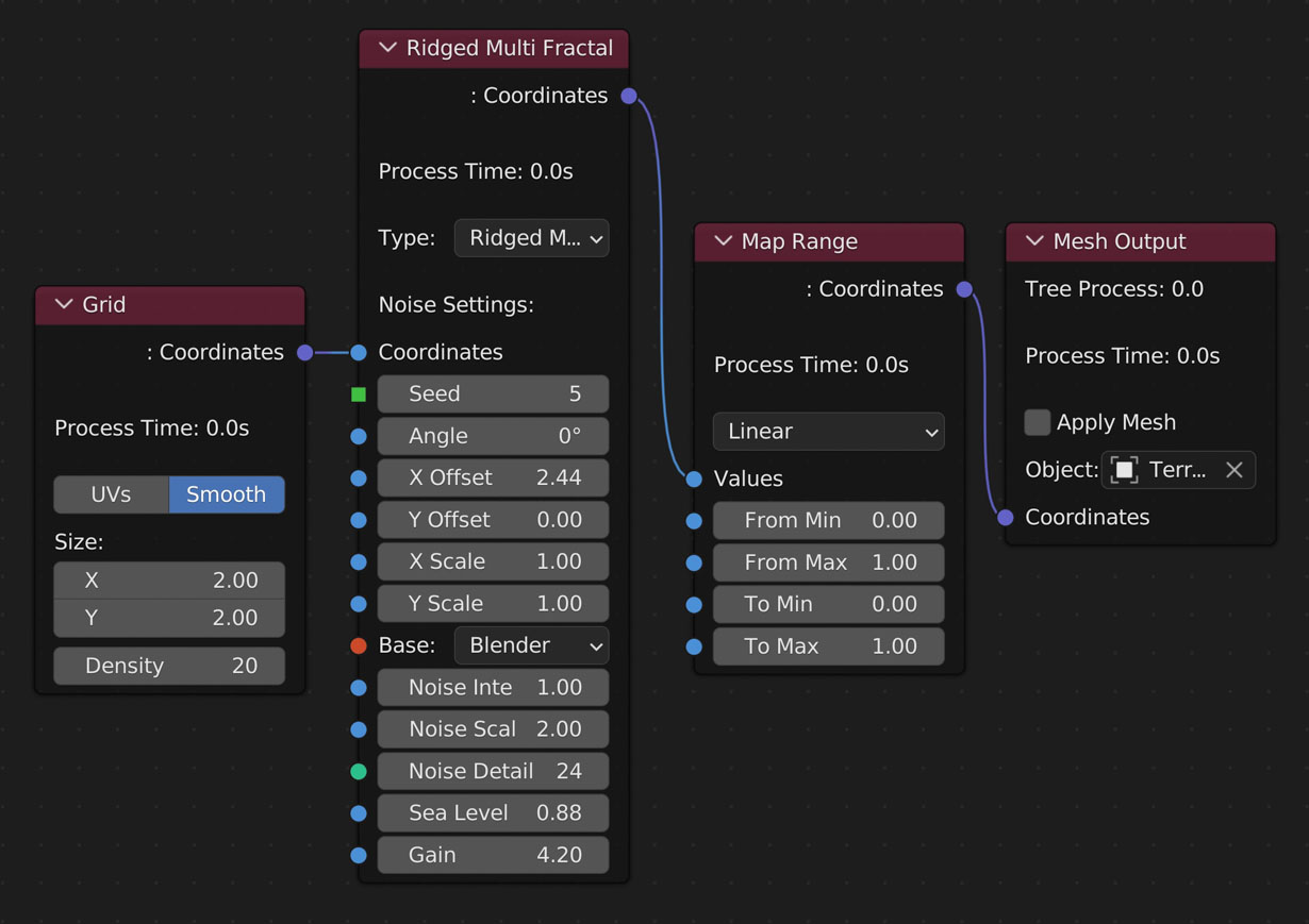
Map Range
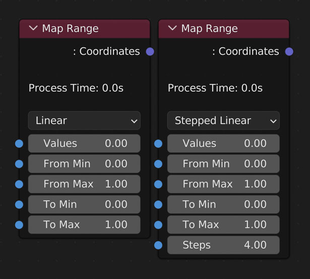
Linearly remap Value.
- Value
- Link values you’d like to affect here
- Interpolation Type
- Linear
- Stepped Linear
- Smooth Step
- Smoother Step
- From Min
- All values less than and equal to this value will be remapped to To Min
- From Max
- All values greater than and equal to this value will be remapped to To Max
- To Min
- The smallest value you want to export
- To Max
- The largest value you want to export
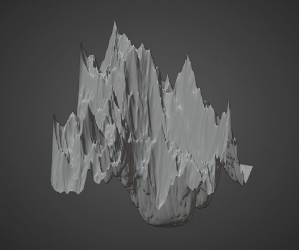
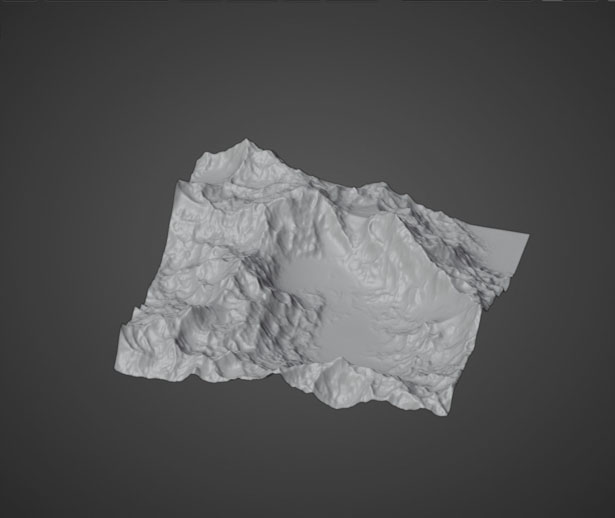
Example:
Linearly remap Value.
- Value
- Link values you’d like to affect here
- Interpolation Type
- Linear
- Stepped Linear
- Smooth Step
- Smoother Step
- From Min
- All values less than and equal to this value will be remapped to To Min
- From Max
- All values greater than and equal to this value will be remapped to To Max
- To Min
- The smallest value you want to export
- To Max
- The largest value you want to export
Example:
Remap 0-1
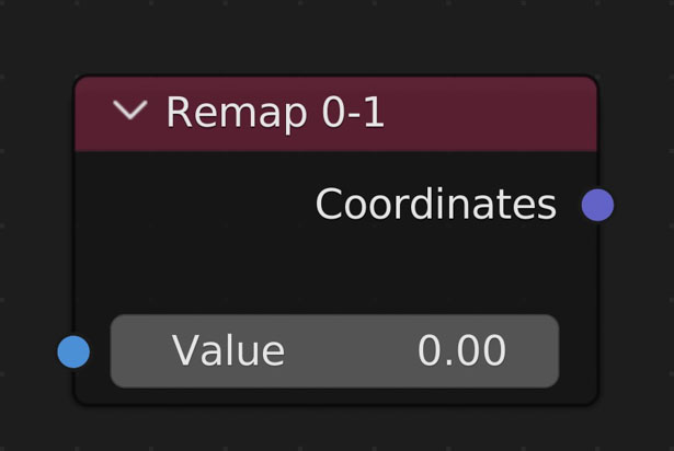
Remaps all values to be between 0 and 1 without clamping.
- Useful for making Vertex Color and Weight maps
Example:
Remaps all values to be between 0 and 1 without clamping.
- Useful for making Vertex Color and Weight maps
Example:
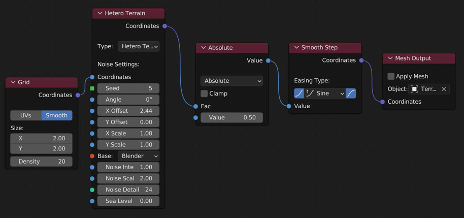
Smooth Step
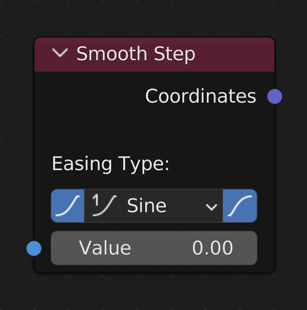
Remaps Value to a given curve
- Ease In
- Ease in with the given curve
- Ease Out
- Ease out with the given curve
- Easing Function
- Sine
- Ease using the sine formula.
- Quadratic
- Ease using a quadratic curve.
- Cubic
- Ease using a cubic curve.
- Quartic
- Ease using a quartic curve.
- Quintic
- Ease using a quintic curve.
- Exponential
- Ease using an exponential curve.
- Circle
- Ease using a circle curve.
- Back
- Ease using a back curve (pushes smallest and largest values up/down a bit respectively.
- Elastic
- Ease using an elastic curve (similar to Back but multiple times).
- Bounce
- Ease using a bounce curve (a curve one might use to animate a bouncing ball).
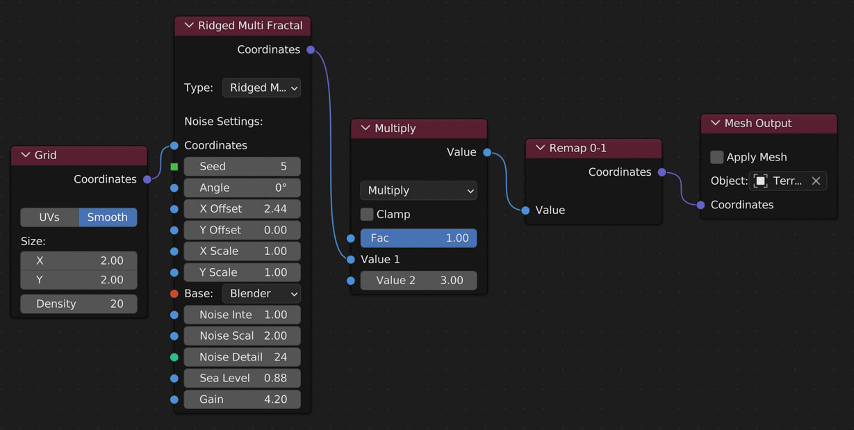
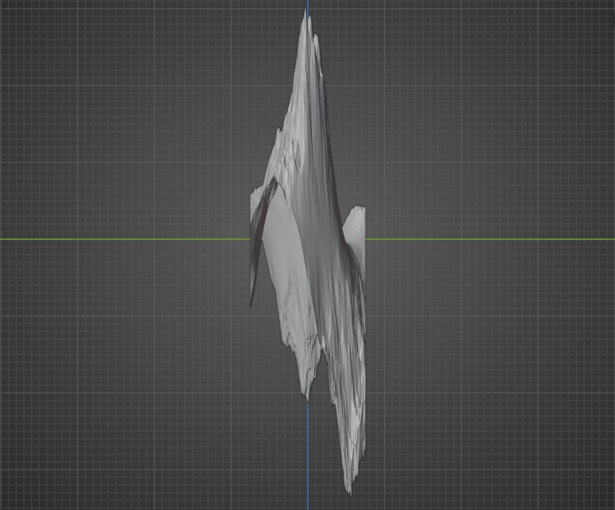
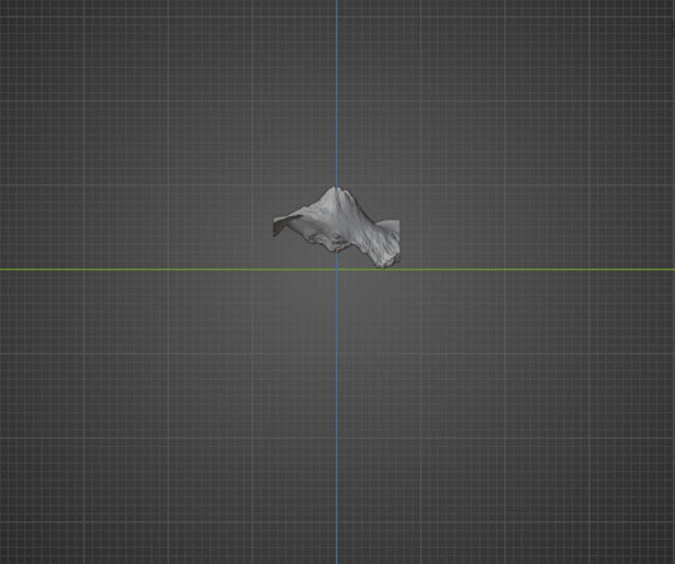
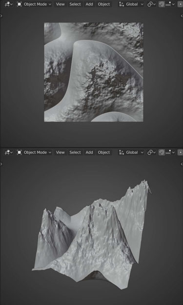
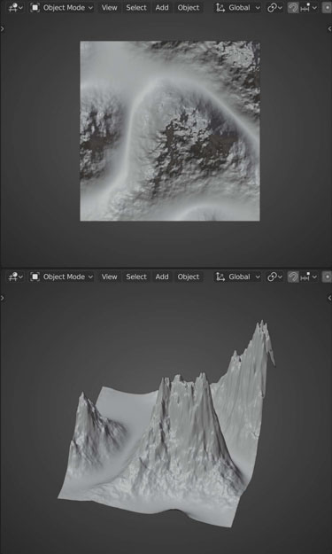
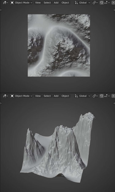
Example:
Remaps Value to a given curve
- Ease In
- Ease in with the given curve
- Ease Out
- Ease out with the given curve
- Easing Function
- Sine
- Ease using the sine formula.
- Quadratic
- Ease using a quadratic curve.
- Cubic
- Ease using a cubic curve.
- Quartic
- Ease using a quartic curve.
- Quintic
- Ease using a quintic curve.
- Exponential
- Ease using an exponential curve.
- Circle
- Ease using a circle curve.
- Back
- Ease using a back curve (pushes smallest and largest values up/down a bit respectively.
- Elastic
- Ease using an elastic curve (similar to Back but multiple times).
- Bounce
- Ease using a bounce curve (a curve one might use to animate a bouncing ball).
Example:
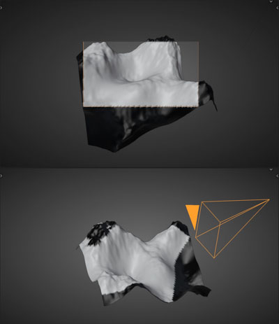
Camera Mask
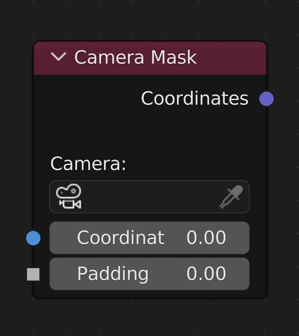
Results in a map of values either '0' or '1'. '0' means the vertex is not visible by the selected camera. '1' means the vertex is visible by the selected camera. Useful for mixing or creating vertex groups for efficient particle placement
- Camera
- The camera to use for visibility
- Coordinates
- Connect the output of the nodes you’d like to use for creating a mask here
- Padding
- Expand the mask beyond the camera bounds.
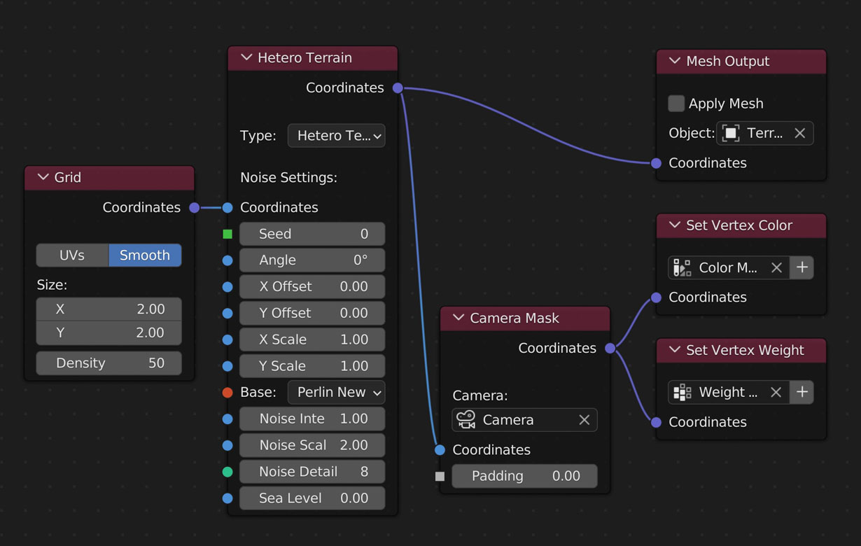
Results Example:
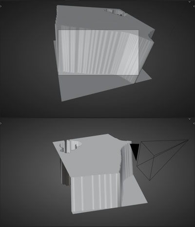
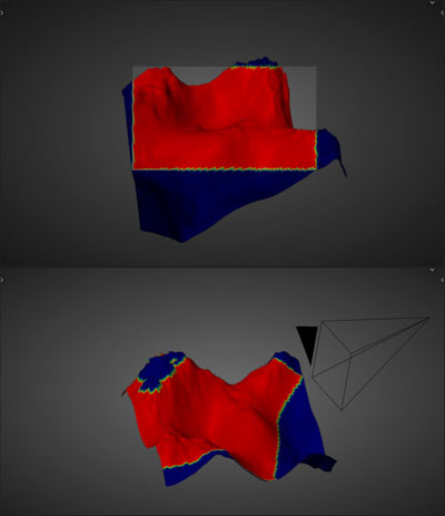
Padding Example:
Update Example:
When a Camera Mask node is selected in the NodeScapes node tree and its chosen camera is moved or its lens/render dimensions change the node will update with each change
Results in a map of values either '0' or '1'. '0' means the vertex is not visible by the selected camera. '1' means the vertex is visible by the selected camera. Useful for mixing or creating vertex groups for efficient particle placement
- Camera
- The camera to use for visibility
- Coordinates
- Connect the output of the nodes you’d like to use for creating a mask here
- Padding
- Expand the mask beyond the camera bounds.
Results Example:
Padding Example:
Update Example:
When a Camera Mask node is selected in the NodeScapes node tree and its chosen camera is moved or its lens/render dimensions change the node will update with each change
Normal Mask
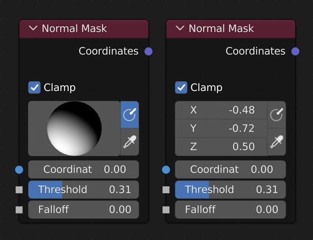
Results in a map of values from 0-infinity relative to how close each vertices' normal is to the target normal and the threshold value
- Clamp
- Values higher than 1 and lower than 0 are ignored and set to either 1 or 0 respectively
- Target Normal
- This is the large sphere in the node
- Click and drag to rotate the sphere in order to choose the normal value. Default value is a normal facing directly up, usually meaning a flat surface
- Show Normal Sphere
- Display the target normal as a sphere to easily rotate the normal
- When off the target normal is displayed as 3 float values
- Normal Picker
- Click a place on the object to choose the normal in that area
- Coordinates
- Connect the output of the nodes you’d like to use for creating a mask here
- Threshold
- How lenient to be when including normal values close to the targeted normal
- Falloff
- How far from the target normal + threshold value to fade out the mask
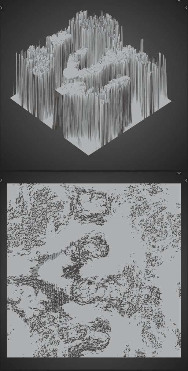
Example:
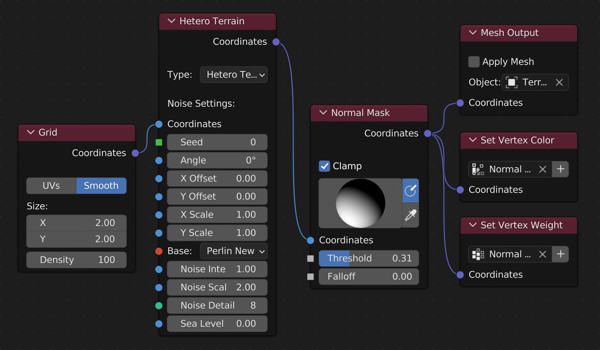
The following images are all using the above layout
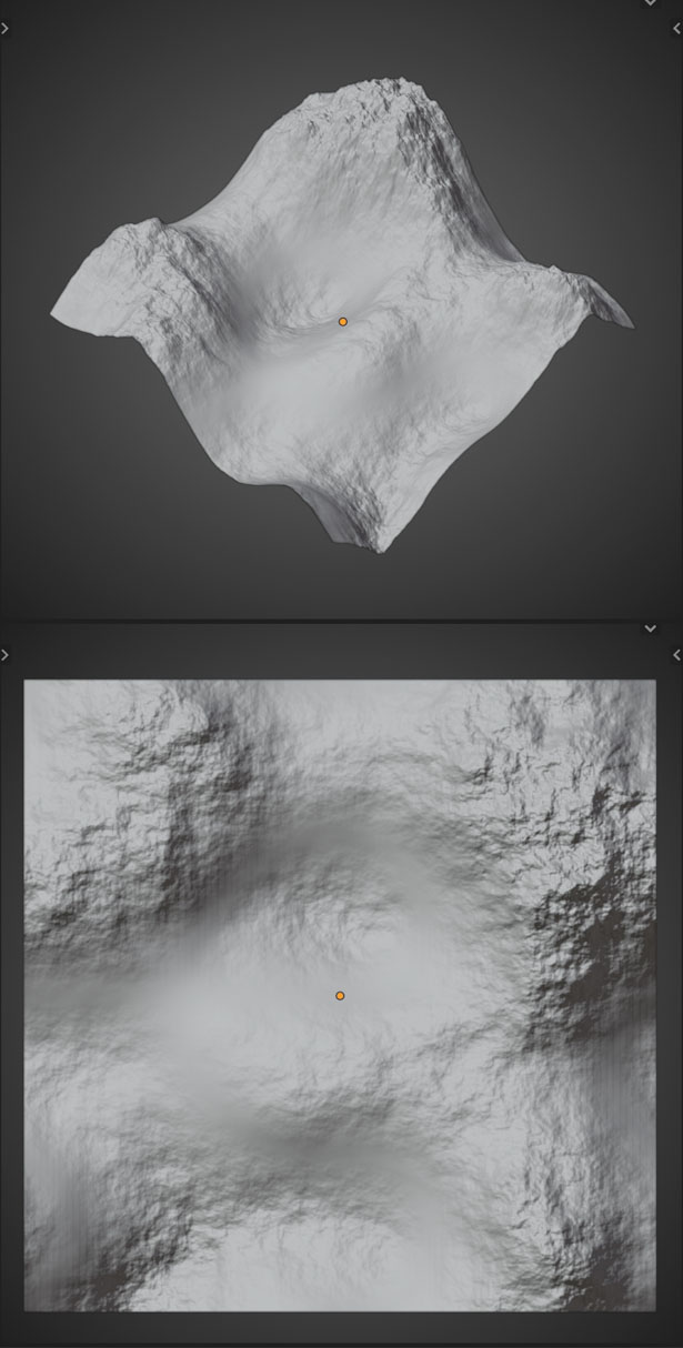
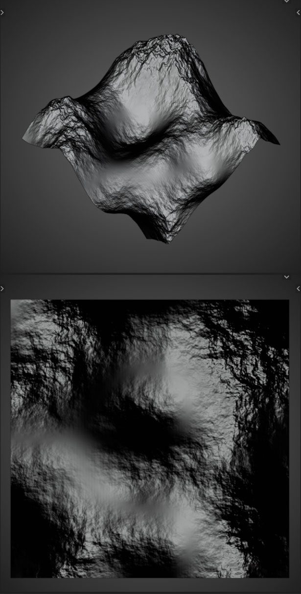
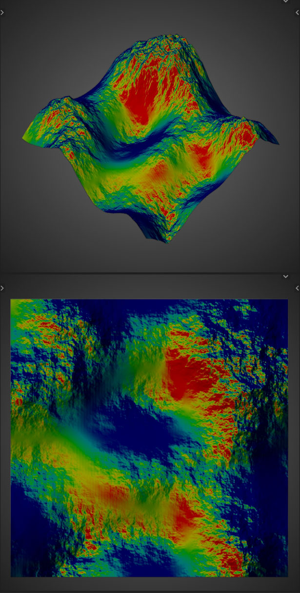
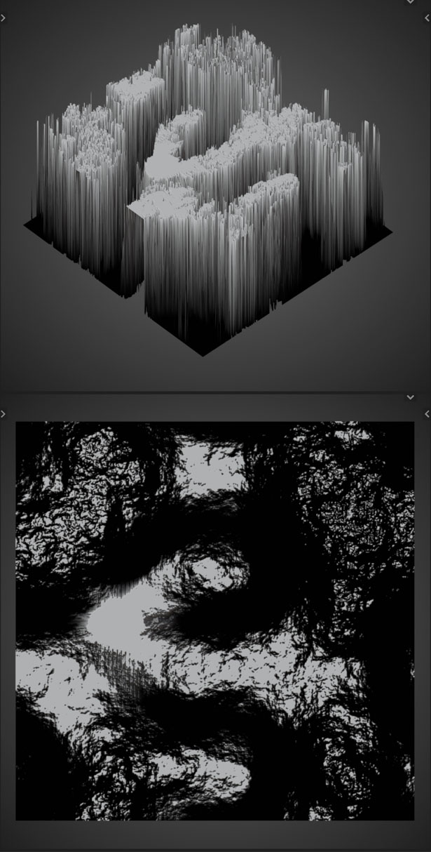
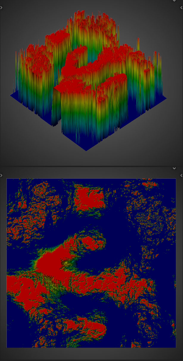
The following images are all using the above layout but with the Normal Mask coordinates connected to the Mesh Output instead of the Hetero Terrain Noise node showing how you can use the output of the Normal Mask for multiple resluts
Results in a map of values from 0-infinity relative to how close each vertices' normal is to the target normal and the threshold value
- Clamp
- Values higher than 1 and lower than 0 are ignored and set to either 1 or 0 respectively
- Target Normal
- This is the large sphere in the node
- Click and drag to rotate the sphere in order to choose the normal value. Default value is a normal facing directly up, usually meaning a flat surface
- Show Normal Sphere
- Display the target normal as a sphere to easily rotate the normal
- When off the target normal is displayed as 3 float values
- Normal Picker
- Click a place on the object to choose the normal in that area
- Coordinates
- Connect the output of the nodes you’d like to use for creating a mask here
- Threshold
- How lenient to be when including normal values close to the targeted normal
- Falloff
- How far from the target normal + threshold value to fade out the mask
Example:
The following images are all using the above layout
The following images are all using the above layout but with the Normal Mask coordinates connected to the Mesh Output instead of the Hetero Terrain Noise node showing how you can use the output of the Normal Mask for multiple resluts
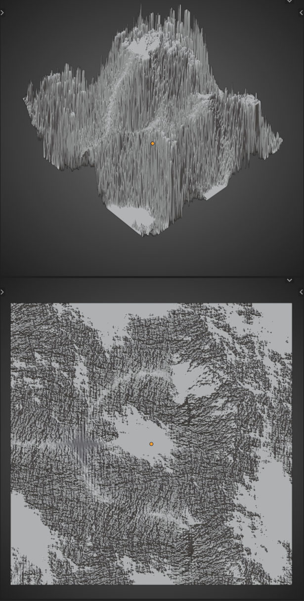
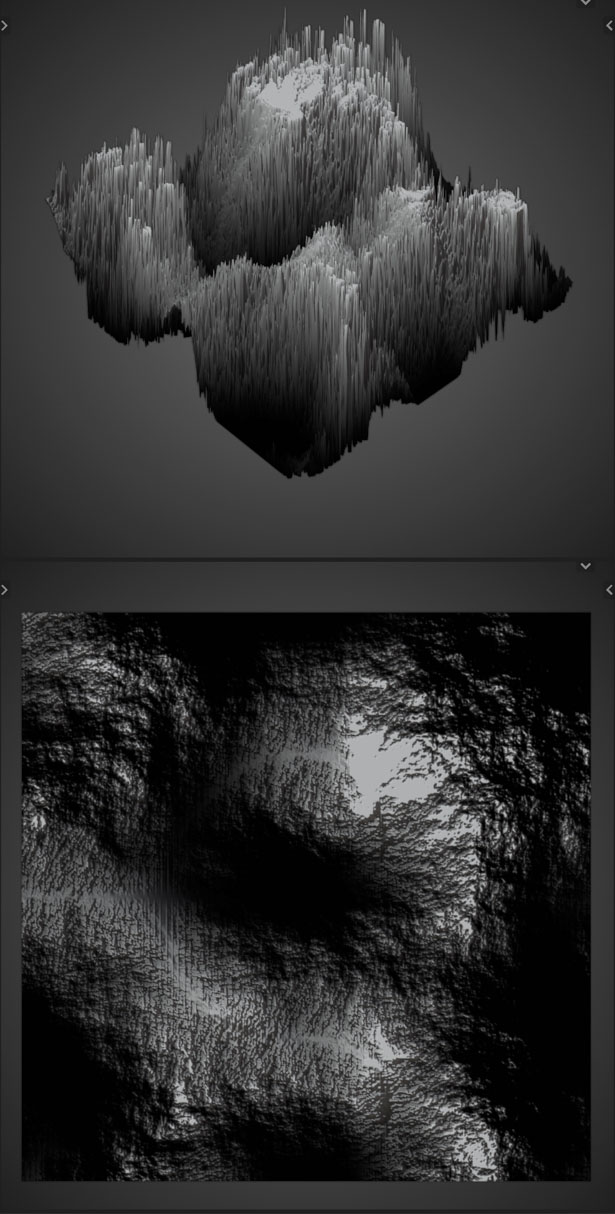
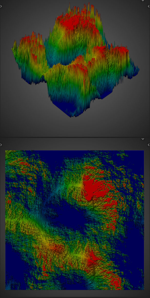
Slope Mask
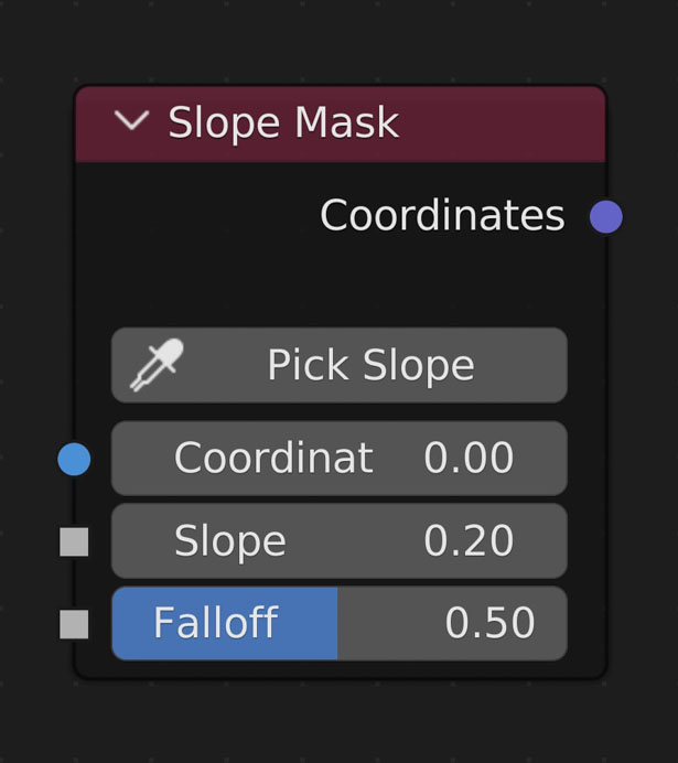
Results in a map of values from 0-infinity relative to how close each vertices' slope is to the Target Slope and the Blend Amount
- Pick Slope
- Click a place on the object to choose the slope in that area
- Coordinates
- Connect the output of the nodes you’d like to use for creating a mask here
- Target Slope
- How great of a slope to include in the map
- Slope is how steep the terrain is at each vertex
- Effectively this is the Normal Mask but doesn't care about direction, only slope
- Falloff
- How lenient to be when including slope values close to the targeted slope
Example:
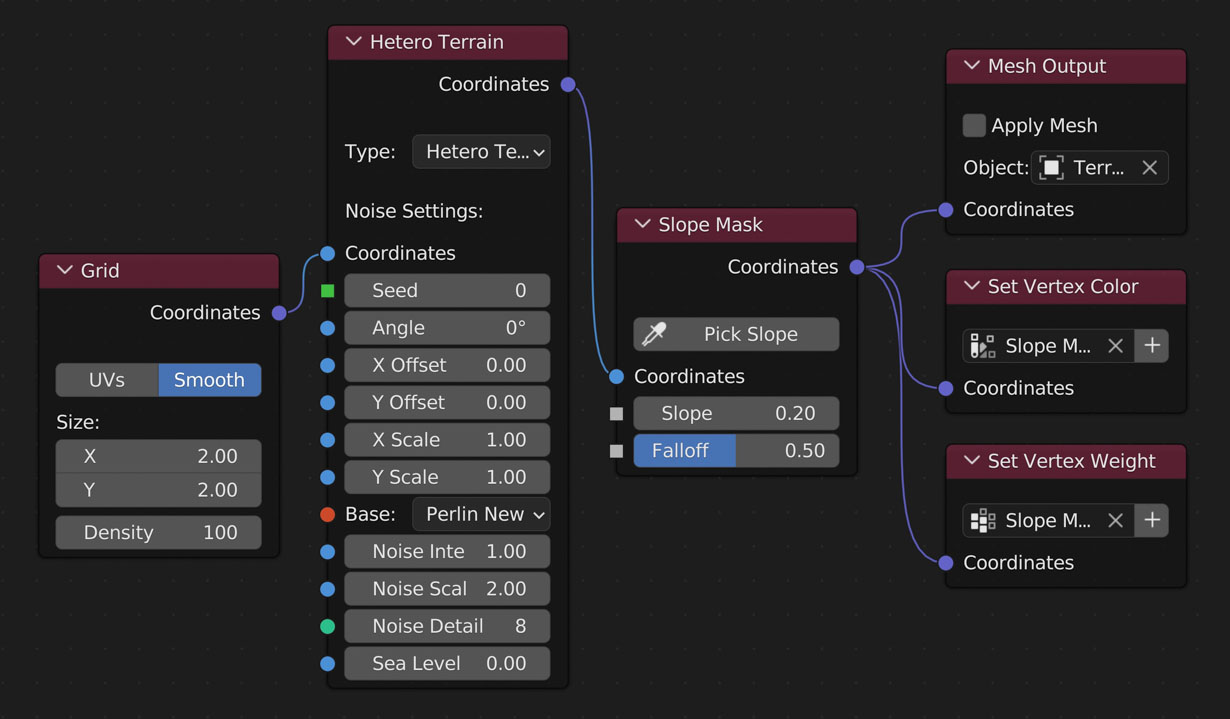
The following images are all using the above layout
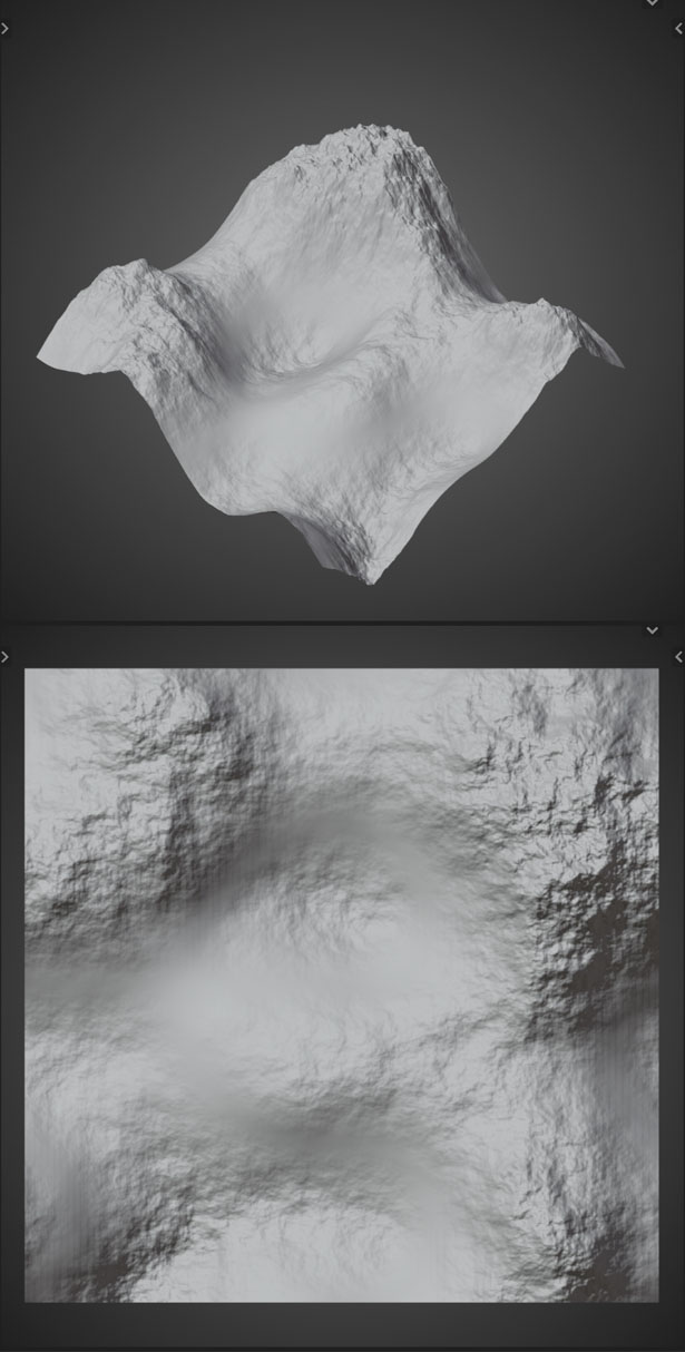
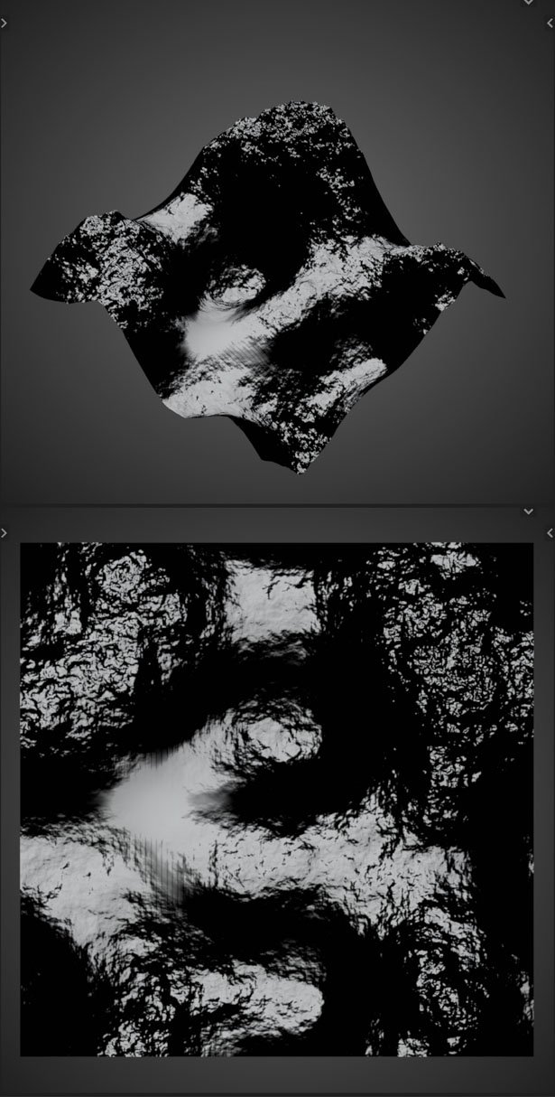
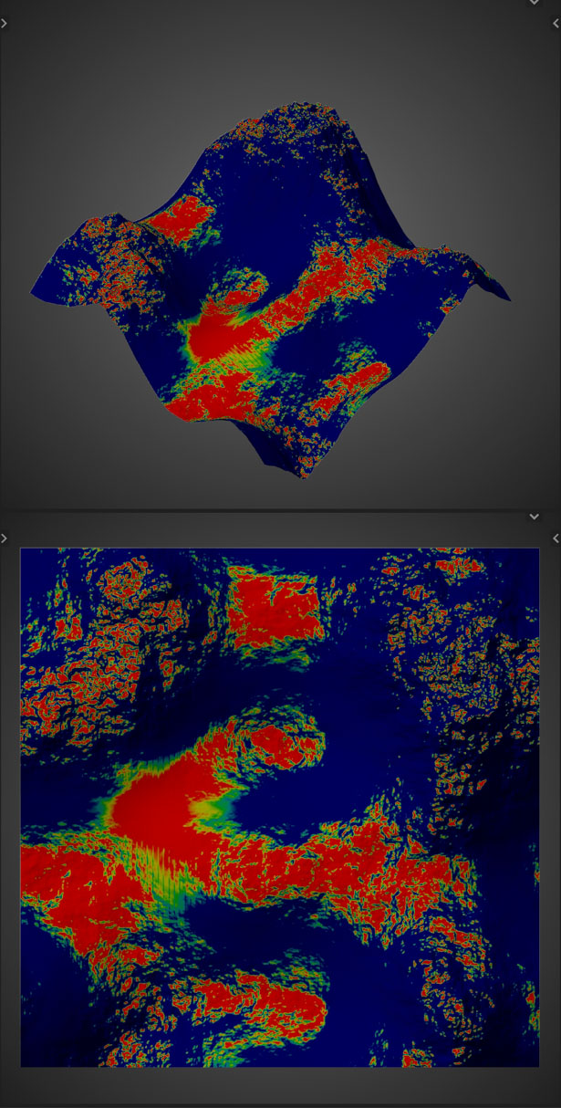
The following images are all using the above layout but with the Slope Mask coordinates connected to the Mesh Output instead of the Hetero Terrain Noise node showing how you can use the output of the Slope Mask for multiple resluts
Results in a map of values from 0-infinity relative to how close each vertices' slope is to the Target Slope and the Blend Amount
- Pick Slope
- Click a place on the object to choose the slope in that area
- Coordinates
- Connect the output of the nodes you’d like to use for creating a mask here
- Target Slope
- How great of a slope to include in the map
- Slope is how steep the terrain is at each vertex
- Effectively this is the Normal Mask but doesn't care about direction, only slope
- Falloff
- How lenient to be when including slope values close to the targeted slope
Example:
The following images are all using the above layout
The following images are all using the above layout but with the Slope Mask coordinates connected to the Mesh Output instead of the Hetero Terrain Noise node showing how you can use the output of the Slope Mask for multiple resluts
Transform
Transform the mesh without affecting the object's transform data
- Translate
- Move the mesh
- Rotate
- Rotate the mesh
- Scale
- Scale the mesh
Transform the mesh without affecting the object's transform data
- Translate
- Move the mesh
- Rotate
- Rotate the mesh
- Scale
- Scale the mesh
Vertex Edits
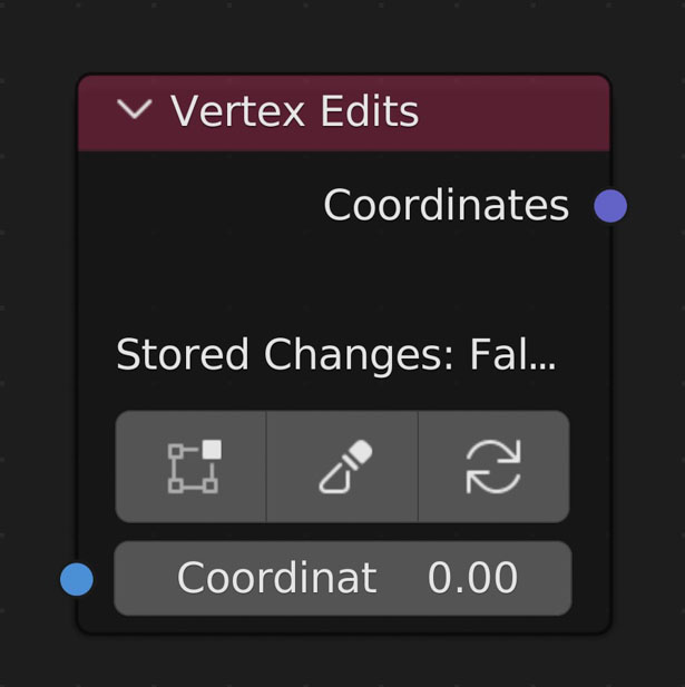
The 'Vertex Edits' node allows you to save manual edits to the geometry from Sculpt Mode or Edit Mode and keep adding and changing node settings.
- Save From Edit Mode
- Enter into Edit Mode to make changes. Only changes to the Z axis will be saved. The mesh will be reverted and changes not saved if an vertices or edges are added during this mode.
- Save From Sculpt Mode
- Enter into Sculpt Mode to make changes. Only changes to the Z axis will be saved. Do not turn on Dynamic Topology or else the mesh will be reverted and any changes unsaved.
- Clear Vertex Edits
- Clicking this button will clear the edits saved to this node
Saving Edits:
Changes are saved when clicking either of the Save from Mode buttons which enters into its respective mode for changes to happen. Once Object Mode has been re-entered the new coordinates are compared with the original coordinates and the difference is added to what was saved previously.
- Each Vertex Edits node can save a new and completely different edit.
- The mesh will be updated to the point the Vertex Edits node exists in the tree. So what is visible in Object Mode may change once Save from Mode has been clicked
- Making changes to the Grid node may cause errors. To fix these errors go back to your original density and size OR clear the edits and do them again.